Quick start guide

In this guide i am going describe how to use the FRI python library to analyse arbitrary datasets.

(This guide is a copy of the official documentation found here)

Installation

Stable

Fri can be installed via the Python Package Index (PyPI).

If you have pip installed just execute the command

pip install fri

to get the newest stable version.

The dependencies should be installed and checked automatically. If you have problems installing please open issue at our tracker.

Development

To install a bleeding edge dev version of FRI you can clone the GitHub repository using

git clone git@github.com:lpfann/fri.git

and then check out the dev branch: git checkout dev.

To check if everything works as intented you can use pytest to run the unit tests. Just run the command

pytest

in the main project folder

# For the purpose of viewing this notebook online we install the library directly with pip
!pip install fri

Requirement already satisfied: fri in /home/lpfannschmidt/workbench/fri (3.4.0+2.g1eb5429.dirty)
Requirement already satisfied: numpy in /home/lpfannschmidt/anaconda3/lib/python3.7/site-packages (from fri) (1.15.1)
Requirement already satisfied: scipy>=0.19 in /home/lpfannschmidt/anaconda3/lib/python3.7/site-packages (from fri) (1.1.0)
Requirement already satisfied: scikit-learn>=0.18 in /home/lpfannschmidt/anaconda3/lib/python3.7/site-packages (from fri) (0.19.2)
Requirement already satisfied: cvxpy==1.0.8 in /home/lpfannschmidt/anaconda3/lib/python3.7/site-packages (from fri) (1.0.8)
Requirement already satisfied: ecos==2.0.5 in /home/lpfannschmidt/anaconda3/lib/python3.7/site-packages (from fri) (2.0.5)
Requirement already satisfied: matplotlib in /home/lpfannschmidt/anaconda3/lib/python3.7/site-packages (from fri) (2.2.3)
Requirement already satisfied: scs>=1.1.3 in /home/lpfannschmidt/anaconda3/lib/python3.7/site-packages (from cvxpy==1.0.8->fri) (2.0.2)
Requirement already satisfied: toolz in /home/lpfannschmidt/anaconda3/lib/python3.7/site-packages (from cvxpy==1.0.8->fri) (0.9.0)
Requirement already satisfied: multiprocess in /home/lpfannschmidt/anaconda3/lib/python3.7/site-packages (from cvxpy==1.0.8->fri) (0.70.6.1)
Requirement already satisfied: osqp in /home/lpfannschmidt/anaconda3/lib/python3.7/site-packages (from cvxpy==1.0.8->fri) (0.4.1)
Requirement already satisfied: fastcache in /home/lpfannschmidt/anaconda3/lib/python3.7/site-packages (from cvxpy==1.0.8->fri) (1.0.2)
Requirement already satisfied: six in /home/lpfannschmidt/anaconda3/lib/python3.7/site-packages (from cvxpy==1.0.8->fri) (1.11.0)
Requirement already satisfied: cycler>=0.10 in /home/lpfannschmidt/anaconda3/lib/python3.7/site-packages (from matplotlib->fri) (0.10.0)
Requirement already satisfied: pyparsing!=2.0.4,!=2.1.2,!=2.1.6,>=2.0.1 in /home/lpfannschmidt/anaconda3/lib/python3.7/site-packages (from matplotlib->fri) (2.2.0)
Requirement already satisfied: python-dateutil>=2.1 in /home/lpfannschmidt/anaconda3/lib/python3.7/site-packages (from matplotlib->fri) (2.7.3)
Requirement already satisfied: pytz in /home/lpfannschmidt/anaconda3/lib/python3.7/site-packages (from matplotlib->fri) (2018.5)
Requirement already satisfied: kiwisolver>=1.0.1 in /home/lpfannschmidt/anaconda3/lib/python3.7/site-packages (from matplotlib->fri) (1.0.1)
Requirement already satisfied: dill>=0.2.8.1 in /home/lpfannschmidt/anaconda3/lib/python3.7/site-packages (from multiprocess->cvxpy==1.0.8->fri) (0.2.8.2)
Requirement already satisfied: future in /home/lpfannschmidt/anaconda3/lib/python3.7/site-packages (from osqp->cvxpy==1.0.8->fri) (0.16.0)
Requirement already satisfied: setuptools in /home/lpfannschmidt/anaconda3/lib/python3.7/site-packages (from kiwisolver>=1.0.1->matplotlib->fri) (40.2.0)

Using FRI

Now we showcase the workflow of using FRI on a simple classification problem.

Data

To have something to work with, we need some data first. fri includes a generation method for binary classification and regression data.

In our case we need some classification data.

from fri import genClassificationData

We want to create a small set with a few features.

Because we want to showcase the all-relevant feature selection, we generate multiple strongly and weakly relevant features.

n = 100
features = 6
strongly_relevant = 2
weakly_relevant = 2

X,y = genClassificationData(n_samples=n,
                            n_features=features,
                            n_strel=strongly_relevant,
                            n_redundant=weakly_relevant,
                            random_state=123)

Generating dataset with d=6,n=100,strongly=2,weakly=2, partition of weakly=None

The method also prints out the parameters again.

X.shape

(100, 6)

We created a binary classification set with 6 features of which 2 are strongly relevant and 2 weakly relevant.

Preprocess

Because our method expects mean centered data we need to standardize it first. This centers the values around 0 and deviation to the standard deviation

from sklearn.preprocessing import StandardScaler
X_scaled = StandardScaler().fit_transform(X)

Model

Now we need to creata a Model. We use the FRIClassification class.

For regression one would use FRIRegression

from fri import FRIClassification
fri_model = FRIClassification()

fri_model

FRIClassification(C=None, debug=False, n_resampling=3,
         optimum_deviation=0.001, parallel=False, random_state=None)

We used no parameters for creation so the defaults are active.

C=None means, that FRI itself chooses the regularization parameter C using crossvalidation on a fixed grid.

By default, parallel computation is also disabled but can be enabled using parallel=True.

Fitting to data

Now we can just fit the model to the data using scikit-learn like commands.

fri_model.fit(X_scaled,y)

The resulting feature relevance bounds are saved in the interval_ variable.

fri_model.interval_

array([[0.45993233, 0.46169499],
       [0.26954548, 0.27159876],
       [0.        , 0.25802293],
       [0.        , 0.25802293],
       [0.00516909, 0.00711219],
       [0.00446591, 0.00694219]])

fri_model.interval_.shape

(6, 2)

The bounds are grouped in 2d sublists for each feature.

To acess the relevance bounds for feature 2 we would use

fri_model.interval_[2]

array([0.        , 0.25802293])

The relevance classes are saved in the corresponding variable relevance_classes_:

fri_model.relevance_classes_

array([2, 2, 1, 1, 0, 0])

2 denotes strongly relevant features, 1 weakly relevant and 0 irrelevant.

Plot results

The bounds in numerical form are useful for postprocesing. If we want a human to look at it, we recommend the plot function plot_relevance_bars.

We can also color the bars according to relevance_classes_

# Import plot function
from fri.plot import plot_relevance_bars
import matplotlib.pyplot as plt
%matplotlib inline
# Create new figure, where we can put an axis on
fig, ax = plt.subplots(1, 1,figsize=(6,3))
# plot the bars on the axis, colored according to fri
out = plot_relevance_bars(ax,fri_model.interval_,classes=fri_model.relevance_classes_)

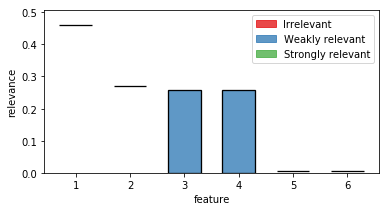
In the plot we can see both strongly relevant features 1 and 2 not allowing much change in their contribution. Feature 3 and 4 are highly correlated and show therefore a big variance. Noise features 5 and 6 show some necessary contribution which can be accounted to numerical instabilities of the solver.

Print internal Parameters

If we want to take at internal parameters, we can use the debug flag in the model creation.

fri_model = FRIClassification(debug=True)

fri_model.fit(X_scaled,y)

loss 0.517120931358002
L1 6.743126681372926
offset 0.32474176019022094
C 1
score 1.0
coef:
[[ 3.10516847]
 [-1.82001413]
 [ 0.86614471]
 [-0.86614471]
 [-0.03919911]
 [-0.03971916]]

This prints out the parameters of the baseline model loss (sum of slack), L1 ($L_1$ norm of weight vector) and offset (from the origin). coef shows the coefficients of the baseline model.

One can also see the best C according to gridsearch and the training score of the model in score.

These values can also be accessed by the object variables.

Print out hyperparameter found by GridSearchCV:

fri_model.tuned_C_

1

or the baseline parameters:

fri_model.optim_L1_

6.743126681372926

Setting constraints manually

Our model also allows to compute relevance bounds when the user sets a given range for the features.

Presets

Presets are encoded using a array in the same shape as the interval_ variable. Each value represents the user given minimum and maximum contribution of the feature. If one would set both values to be the same, we interpret this feature as fixed.

Additionally, entries with np.nan are interpreted as not-set or free.

import numpy as np
preset = np.full_like(fri_model.interval_,np.nan,dtype=np.double)

Now we have a preset array without any constraints:

preset

array([[nan, nan],
       [nan, nan],
       [nan, nan],
       [nan, nan],
       [nan, nan],
       [nan, nan]])

Example

As an example, let us constrain feature 3 from our example to the minimum relevance bound.

Note the different indexing using numpy (3 -> 2)

preset[2] = fri_model.interval_[2, 0]

We use the function constrained_intervals_.

Note: we need to fit the model before we can use this function. We already did that, so we are fine.

constrained_interval = fri_model.constrained_intervals_(preset=preset)

constrained_interval

array([[0.45993233, 0.46169499],
       [0.26954548, 0.27159876],
       [0.        , 0.        ],
       [0.25608488, 0.25802293],
       [0.00516909, 0.00711219],
       [0.00446591, 0.0069422 ]])

Feature 3 is set to its minimum (at 0).

How does it look visually?

fig, ax = plt.subplots(1, 1,figsize=(6,3))
out = plot_relevance_bars(ax, constrained_interval)

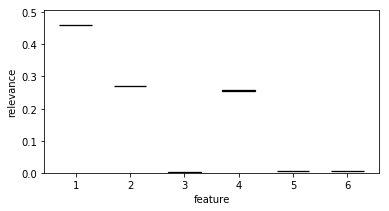
Feature 3 is reduced to its minimum (no contribution).

In turn, its correlated partner feature 4 had to take its maximum contribution.